function VBR = CB_002_2D_HalfSpaceCooling()
%%%%%%%%%%%%%%%%%%%%%%%%%%%%%%%%%%%%%%%%%%%%%%%%%%%%%%%%%%%%%%%%%%%%%%%%%%%
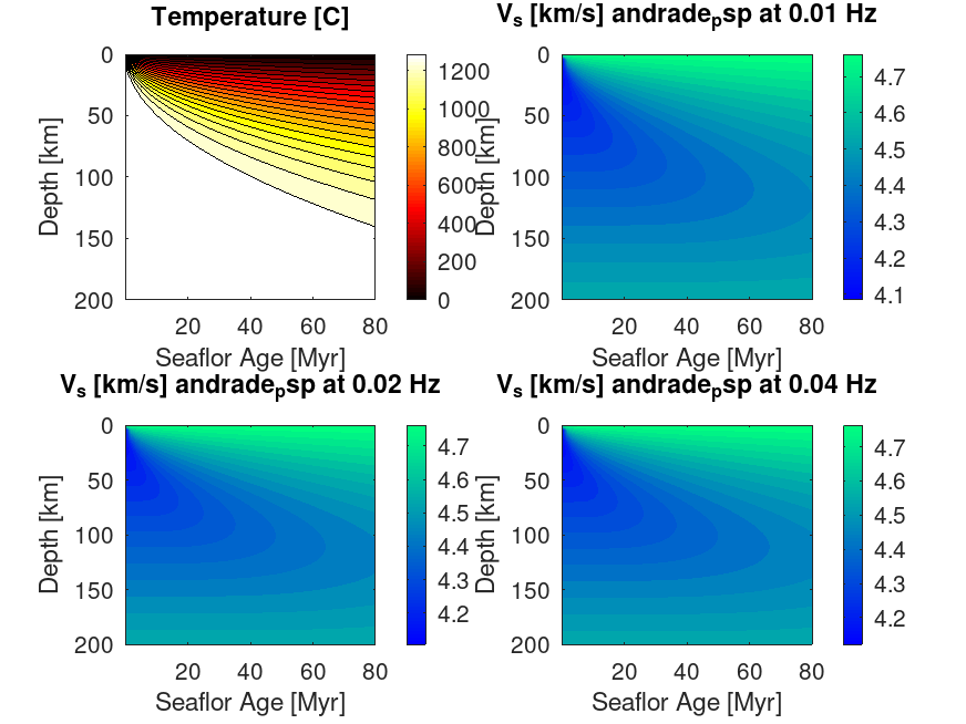
% CB_002_2D_HalfSpaceCooling.m
%
% Calculate seismic properties for a half space cooling model, compares
% results of two anelastic methods.
%%%%%%%%%%%%%%%%%%%%%%%%%%%%%%%%%%%%%%%%%%%%%%%%%%%%%%%%%%%%%%%%%%%%%%%%%%%
%% Set Thermodynamic State Using Half Space Cooling Model %%
%% analytical solution:
%% T(z,t)=T_surf + (T_asth - T_surf) * erf(z / (2sqrt(Kappa * t)))
%% variables defined below
% HF settings
HF.Tsurf_C=0; % surface temperature [C]
HF.Tasth_C=1350; % asthenosphere temperature [C]
HF.V_cmyr=8; % half spreading rate [cm/yr]
HF.Kappa=1e-6; % thermal diffusivity [m^2/s]
HF.rho=3300; % density [kg/m3]
HF.t_Myr=linspace(0,80,50)+1e-12; % seaflor age [Myrs]
HF.z_km=linspace(0,200,55)'; % depth, opposite vector orientation [km]
% HF calculations
HF.s_in_yr=(3600*24*365); % seconds in a year [s]
HF.t_s=HF.t_Myr*1e6*HF.s_in_yr; % plate age [s]
HF.x_km=HF.t_s / (HF.V_cmyr / HF.s_in_yr / 100) / 1000; % distance from ridge [km]
% calculate HF cooling model for each plate age
HF.dT=HF.Tasth_C-HF.Tsurf_C;
HF.T_C=zeros(numel(HF.z_km),numel(HF.x_km));
for HFi_t = 1:numel(HF.t_s)
HF.erf_arg=HF.z_km*1000/(2*sqrt(HF.Kappa*HF.t_s(HFi_t)));
HF.T_C(:,HFi_t)=HF.Tsurf_C+HF.dT * erf(HF.erf_arg);
end
%% Load and set VBR parameters %%
VBR.in.elastic.methods_list={'anharmonic'};
VBR.in.viscous.methods_list={'HK2003'};
VBR.in.anelastic.methods_list={'andrade_psp';'xfit_mxw'};
VBR.in.elastic.anharmonic=Params_Elastic('anharmonic'); % unrelaxed elasticity
VBR.in.elastic.anharmonic.Gu_0_ol = 75.5; % olivine reference shear modulus [GPa]
VBR.in.SV.f = [0.01, 0.02, 0.04, 0.1];% frequencies to calculate at
% copy halfspace model into VBR state variables, adjust units as needed
VBR.in.SV.T_K = HF.T_C+273; % set HF temperature, convert to K
% construct pressure as a function of z, build matrix same size as T_K:
HF.P_z=HF.rho*9.8*HF.z_km*1e3/1e9; %
VBR.in.SV.P_GPa = repmat(HF.P_z,1,numel(HF.t_s)); % pressure [GPa]
% set the other state variables as matrices of same size
sz=size(HF.T_C);
VBR.in.SV.rho = 3300 * ones(sz); % density [kg m^-3]
VBR.in.SV.sig_MPa = 10 * ones(sz); % differential stress [MPa]
VBR.in.SV.phi = 0.0 * ones(sz); % melt fraction
VBR.in.SV.dg_um = 0.01 * 1e6 * ones(sz); % grain size [um]
%% CALL THE VBR CALCULATOR %%
[VBR] = VBR_spine(VBR) ;
%% Build figures %%
if ~vbr_tests_are_running()
% contour T(z,t)
figure()
ax1=subplot(2,2,1);
contourf(HF.t_Myr,HF.z_km,HF.T_C,20)
colormap(ax1,hot)
xlabel('Seaflor Age [Myr]')
ylabel('Depth [km]')
set(gca,'ydir','reverse')
title('Temperature [C]')
colorbar()
% contour shear wave velocity at different frequencies
for i_f=1:3
ax=subplot(2,2,i_f+1);
contourf(HF.t_Myr,HF.z_km,VBR.out.anelastic.andrade_psp.V(:,:,i_f)/1e3,20,'LineColor','none')
colormap(ax,winter);
xlabel('Seaflor Age [Myr]')
ylabel('Depth [km]')
set(gca,'ydir','reverse')
title(['V_s [km/s] andrade_psp at ',num2str(VBR.in.SV.f(i_f)),' Hz'])
colorbar()
end
saveas(gcf,'./figures/CB_002_2D_HalfSpaceCooling.png')
% contour percent difference in shear wave velo between two anelastic methods
% at different frequencies
dV=abs(VBR.out.anelastic.andrade_psp.V-VBR.out.anelastic.xfit_mxw.V);
dV=dV./VBR.out.anelastic.xfit_mxw.V*100;
figure()
for i_f=1:4
subplot(2,2,i_f)
dVmask=(dV(:,:,i_f)>0);
contourf(HF.t_Myr,HF.z_km,(dV(:,:,i_f).*dVmask),100,'LineColor','none')
colormap(hot)
caxis([0,max(max(dV(:,:,i_f)))])
xlabel('Seaflor Age [Myr]')
ylabel('Depth [km]')
set(gca,'ydir','reverse')
maxval=round(max(max(dV(:,:,i_f)))*100)/100;
title([num2str(VBR.in.SV.f(i_f)),' Hz, max(dV)=',num2str(maxval),' percent'])
colorbar()
end
end
end