Quick Start
The following outlines the basic usage for the VBR calculator. Additionally, there are a growing number of examples in Projects/ to illustrate more complex usage, particularly in developing a statistical framework for comparing predicted mechanical properties to observed properties. In general, the flow is to:
- Initialize VBR
- Set Methods List
- Specify State Variables
- Adjust Parameters (optional)
- Run the VBR Calculator
- Extract results
0. The VBR structure
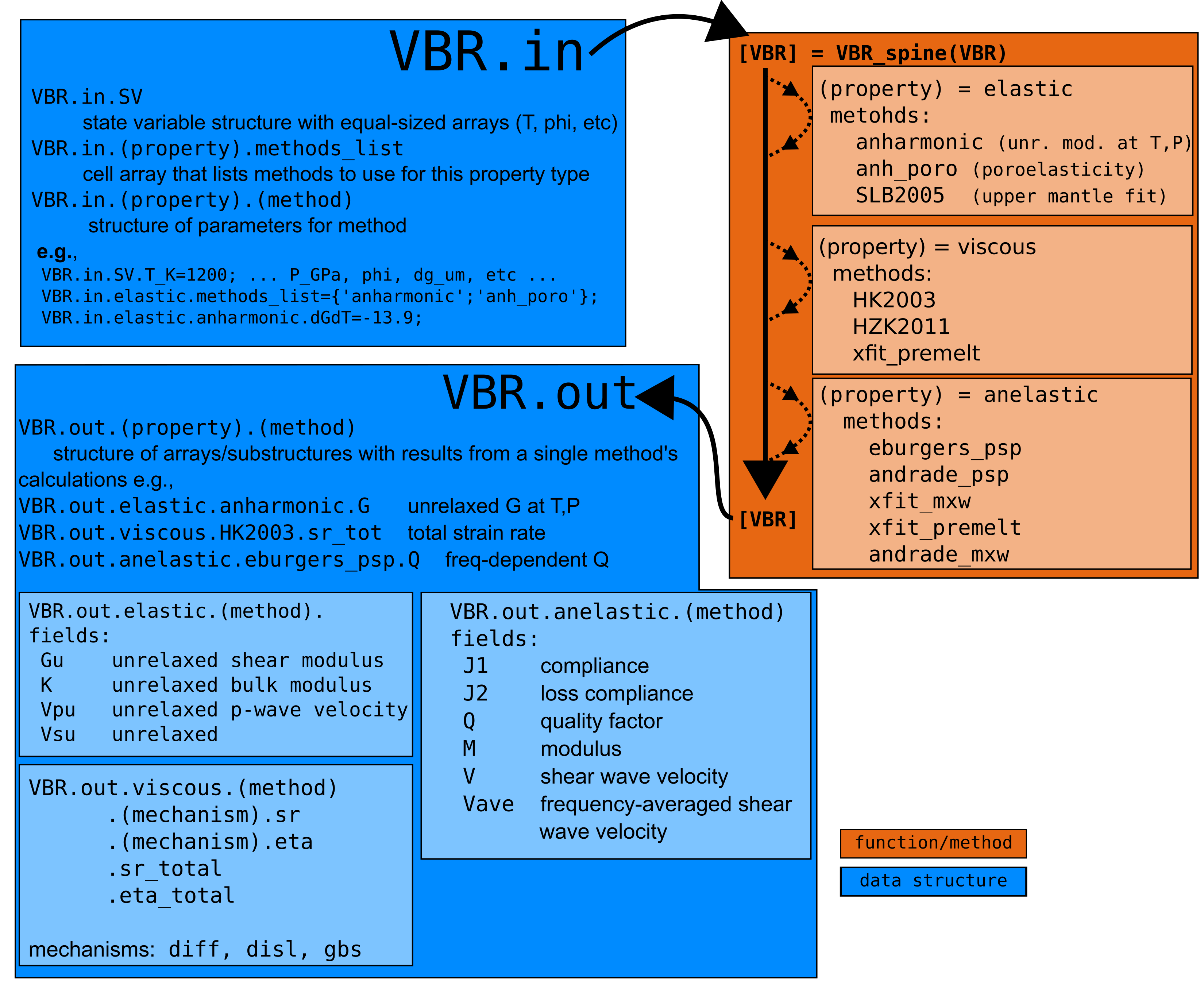
The VBR Calculator is built around MATLAB structures. All direction and data is stored in the VBR structure, which gets passed around to where it needs to go. VBR.in contains the user’s input. VBR.out contains the results of any calculations.
1. Initialize VBR
To start, add the top level directory to your MATLAB path (relative or absolute path) and run vbr_init to add all the required directories to your path:
vbr_path='~/src/vbr/';
addpath(vbr_path)
vbr_init
If desired, you can permanently add the vbr directory to your path and even call vbr_init on opening MATLAB by adding the above lines to the startup.m file (see here for help).
2. Set Methods List
The user must supply a cell array called methods_list for each property for which they want to calculate (see here for more on available methods):
VBR.in.elastic.methods_list={'anharmonic';'anh_poro';};
VBR.in.viscous.methods_list={'HK2003','HZK2011'};
VBR.in.anelastic.methods_list={'eburgers_psp';'andrade_psp';'xfit_mxw'};
Each method will have a field in VBR.out beneath the property, e.g.,
VBR.out.elastic.anharmonic
VBR.out.viscous.HK2003
VBR.out.anelastic.eburgers_psp
VBR.out.anelastic.andrade_psp
beneath which there will be fields for the output for the calculations, e.g., VBR.out.anelastic.andrade_psp.Q for quality factor Q (attenuation=Q-1).
After VBR is initialized, a list of available methods can be printed by running VBR_list_methods(). For theoretical background on the different methods, see the accompanying VBR Calculator Manual.
3. Specify the State Variables
The input structure VBR.in.SV contains the state variables that define the conditions at which you want to apply the methods. The following fields MUST be defined:
%  frequencies to calculate at
   VBR.in.SV.f = logspace(-2.2,-1.3,4); % [Hz]

%  size of the state variable arrays. arrays can be any shape
%  but all arays must be the same shape.
   n1 = 1;

   VBR.in.SV.P_GPa = 2 * ones(n1,1); % pressure [GPa]
   VBR.in.SV.T_K = 1473 * ones(n1,1); % temperature [K]
   VBR.in.SV.rho = 3300 * ones(n1,1); % density [kg m^-3]
   VBR.in.SV.sig_MPa = 10 * ones(n1,1); % differential stress [MPa]

   VBR.in.SV.phi = 0.0 * ones(n1,1); % melt fraction
   VBR.in.SV.dg_um = 0.01 * 1e6 * ones(n1,1); % grain size [um]
while the following fields are optional:
%  optional state variables
   VBR.in.SV.chi=1*ones(n1,1); % composition fraction: 1 for olivine, 0 for crust (OPTIONAL, DEFAULT 1)
   VBR.in.SV.Ch2o = 0 * ones(n1,1) ; % water concentration  (OPTIONAL, DEFAULT 0)
All SV arrays must be the same size and shape, except for the frequency VBR.in.SV.f. They can be any length and shape as long as they are the same. Frequency dependent variables store the frequency dependencein an extra dimension of the output. If size(VBR.in.SV.T) is (50,100) and numel(VBR.in.SV.f) is 3, then size(VBR.out.anelastic.eburgers_psp.V) will be (50,100,3).
4. Adjust parameters (optional)
The VBR calculator allows the user to change any parameter they see fit. Parameters are stored in the VBR.in.(property).(method) structure, e.g.:
VBR.in.elastic.anharmonic.Gu_0_ol = 75.5; % olivine reference shear modulus [GPa]
VBR.in.viscous.HZK2011.diff.Q=350e3; % diffusion creep activation energy
The default parameters are stored in vbr/vbrCore/params/ and can be loaded and explored with
VBR.in.elastic.anharmonic=Params_Elastic('anharmonic'); % unrelaxed elasticity
VBR.in.viscous.HZK2011=Params_Viscous('HZK2011'); % HZK2011 params
When changing parameters from those loaded by default, you can either load all the parameters then overwrite them or in most cases you can simply set the parameters without loading the full set of parameters.
5. Run the VBR Calculator
The VBR Calculator executes calculations by passing the VBR structure to the VBR_spine():
[VBR] = VBR_spine(VBR) ;
6. Extract results
Results are stored in VBR.out for each property type and method:
VBR.out.elastic.anharmonic.Vsu % unrelaxed seismic shear wave velocity
VBR.out.anelastic.eburgers_psp.V % anelastic-dependent seismic shear wave velocity
VBR.out.viscous.HZK2011.eta_total % composite steady state creep viscosity
As noted above, any frequency dependence is stored in an additional dimension. For example, if size(VBR.in.SV.T) is (50,100) and numel(VBR.in.SV.f) is 3, then size(VBR.out.anelastic.eburgers_psp.V) will be (50,100,3).
7. Saving results
To save your results, you can manually save the VBR structure as usual in MATLAB. You can, however, also use the VBR_save function:
VBR_save(VBR, "my_vbrc_results.mat")
This function is useful to ensure that the VBR structure is saved in a standardized way, which at present is mainly useful for loading VBRc output in the Python wrapper of the VBRc, pyVBRc(link).
Additionally, VBR_save allows you to easily exclude the VBR.in.SV structure from the saved file:
VBR_save(VBR, "my_vbrc_results_without_SV.mat", 1)
This can be useful if you wish to save disk space and instead reconstruct your state variables on re-load (which you must do manually!).