CB_003_JF10.m

output figures

'CB_003_JF10'
%%%%%%%%%%%%%%%%%%%%%%%%%%%%%%%%%%%%%%%%%%%%%%%%%%%%%%%%%%%%%%%%%%%%%%%%%%%
% CB_003_JF10.m
%
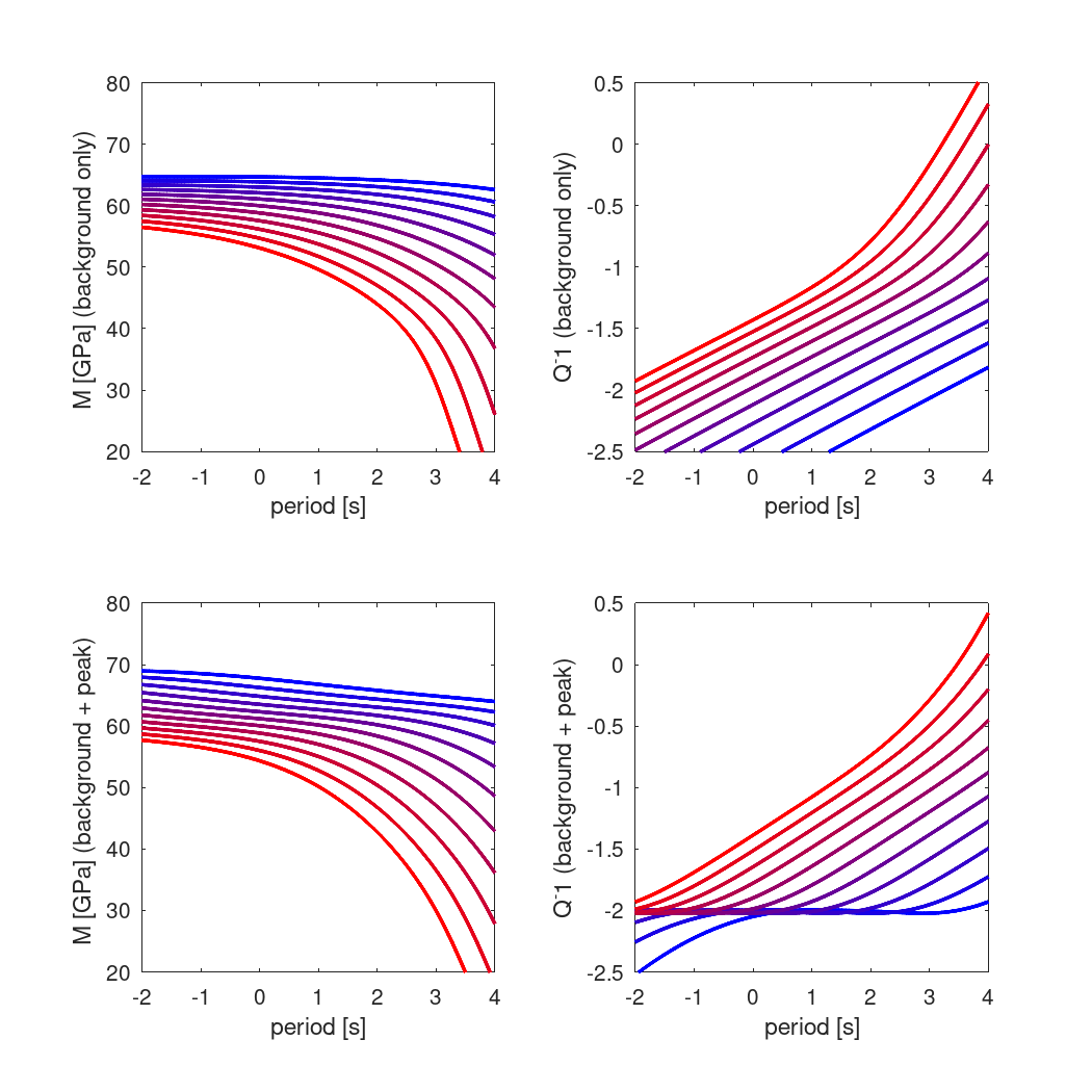
%  Reproduces figures 1a-1d from JF10: moduli and Qinv vs period for
%  a single sample, #6585, using coefficients for the single sample fit
%  in table 1 of JF10.
%%%%%%%%%%%%%%%%%%%%%%%%%%%%%%%%%%%%%%%%%%%%%%%%%%%%%%%%%%%%%%%%%%%%%%%%%%%

%% put VBR in the path %%
  clear; close all;
  path_to_top_level_vbr='../../';
  addpath(path_to_top_level_vbr)
  vbr_init

%%  write method list %%
  VBR.in.elastic.methods_list={'anharmonic'};
  VBR.in.anelastic.methods_list={'eburgers_psp';'andrade_psp'};

%%  load anharmonic parameters, adjust Gu_0_ol %%
  % all params in ../vbr/vbrCore/params/ will be loaded in call to VBR spine,
  % but you can load them here and adjust any one of them (rather than changing
  % those parameter files).
  VBR.in.elastic.anharmonic=Params_Elastic('anharmonic'); % unrelaxed elasticity
  VBR.in.anelastic.eburgers_psp=Params_Anelastic('eburgers_psp');

  % use the single sample background only fit:
  VBR.in.anelastic.eburgers_psp.eBurgerMethod='s6585_bg_only'; % 'bg_only' or 'bg_peak' or 's6585_bg_only'

  % JF10 have Gu_0=62.5 GPa, but that's at 900 Kelvin and 0.2 GPa,
  % so set Gu_0_ol s.t. it ends up at 62.5 at those conditions
  dGdT=VBR.in.elastic.anharmonic.dG_dT;
  dGdP=VBR.in.elastic.anharmonic.dG_dP;
  Tref=VBR.in.elastic.anharmonic.T_K_ref;
  Pref=VBR.in.elastic.anharmonic.P_Pa_ref/1e9;
  GUJF10=VBR.in.anelastic.eburgers_psp.s6585_bg_only.G_UR;
  VBR.in.elastic.anharmonic.Gu_0_ol = GUJF10 - (900+273-Tref) * dGdT/1e9 - (0.2-Pref)*dGdP; % olivine reference shear modulus [GPa]

  % frequencies to calculate at
  VBR.in.SV.f = 1./logspace(-2,4,100);

%% Define the Thermodynamic State %%
  VBR.in.SV.T_K=700:50:1200;
  VBR.in.SV.T_K=VBR.in.SV.T_K+273;
  sz=size(VBR.in.SV.T_K); % temperature [K]

  % remaining state variables
  VBR.in.SV.dg_um=3.1*ones(sz);
  VBR.in.SV.P_GPa = 0.2 * ones(sz); % pressure [GPa]
  VBR.in.SV.rho = 3300 * ones(sz); % density [kg m^-3]
  VBR.in.SV.sig_MPa = 10 * ones(sz); % differential stress [MPa]
  VBR.in.SV.phi = 0.0 * ones(sz); % melt fraction

%% call VBR_spine %%
  [VBR] = VBR_spine(VBR) ;

%% adjust VBR input to include dissipation peak in the eburgers method %%
  VBR.in.anelastic.eburgers_psp.eBurgerFit='s6585_bg_peak';

  % this fit has a slightly different ref modulus, adjust it again:
  GUJF10=VBR.in.anelastic.eburgers_psp.s6585_bg_peak.G_UR;
  VBR.in.elastic.anharmonic.Gu_0_ol = GUJF10 - (900+273-Tref) * dGdT/1e9 - (0.2-Pref)*dGdP;

%% Call VBR_spine again %%
  [VBR_with_peak] = VBR_spine(VBR) ;

%% build figure %%
  figure('PaperPosition',[0,0,7,7],'PaperPositionMode','manual');

  for iTemp = 1:numel(VBR.in.SV.T_K)

    M_bg=squeeze(VBR.out.anelastic.eburgers_psp.M(1,iTemp,:)/1e9);
    M_bg_peak=squeeze(VBR_with_peak.out.anelastic.eburgers_psp.M(1,iTemp,:)/1e9);
    Q_bg=squeeze(VBR.out.anelastic.eburgers_psp.Qinv(1,iTemp,:));
    Q_bg_peak=squeeze(VBR_with_peak.out.anelastic.eburgers_psp.Qinv(1,iTemp,:));
    logper=log10(1./VBR.in.SV.f);
    R=(iTemp-1) / (numel(VBR.in.SV.T_K)-1);
    B=1 - (iTemp-1) / (numel(VBR.in.SV.T_K)-1);

    subplot(2,2,1)
    hold on
    plot(logper,M_bg,'color',[R,0,B],'LineWidth',2);
    ylabel('M [GPa] (background only) '); xlabel('period [s]')
    ylim([20,80])

    subplot(2,2,2)
    hold on
    plot(logper,log10(Q_bg),'color',[R,0,B],'LineWidth',2);
    ylabel('Q^-1 (background only)'); xlabel('period [s]')
    ylim([-2.5,0.5])

    subplot(2,2,3)
    hold on
    plot(logper,M_bg_peak,'color',[R,0,B],'LineWidth',2);
    ylabel('M [GPa] (background + peak) '); xlabel('period [s]')
    ylim([20,80])

    subplot(2,2,4)
    hold on
    plot(logper,log10(Q_bg_peak),'color',[R,0,B],'LineWidth',2);
    ylabel('Q^-1 (background + peak)'); xlabel('period [s]')
    ylim([-2.5,0.5])
  end
  for ip = 1:4
    subplot(2,2,ip); box on;
  end
  saveas(gcf,'./figures/CB_003_JF10.png')
CB_003_JF10.m

output figures

contents
