CB_008_anharmonic_Gu0.m

output figures

contents

function VBR = CB_008_anharmonic_Gu0()
  %%%%%%%%%%%%%%%%%%%%%%%%%%%%%%%%%%%%%%%%%%%%%%%%%%%%%%%%%%%%%%%%%%%%%%%%%%%
  % CB_008_anharmonic_Gu0.m
  %
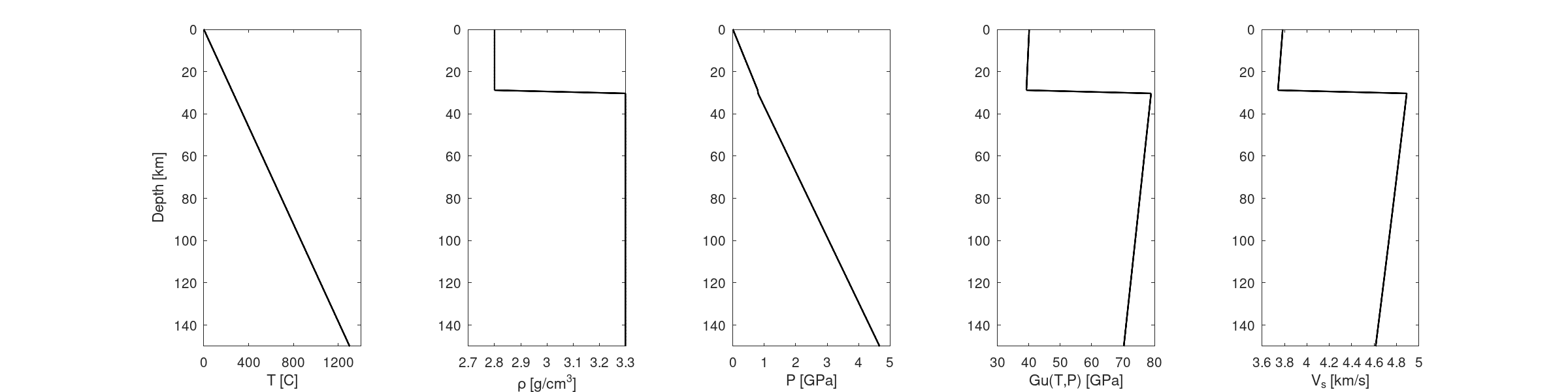
  %   Example of including a depth dependence with a low density crust
  %%%%%%%%%%%%%%%%%%%%%%%%%%%%%%%%%%%%%%%%%%%%%%%%%%%%%%%%%%%%%%%%%%%%%%%%%%%

  %% set depth array and temperature profile %%
  depth_km=linspace(0,150,100);
  VBR.in.SV=struct();
  VBR.in.SV.T_K = 1300 * depth_km/max(depth_km) +273; % temperature [K]

  %% set and calculate density and pressure with a crust %%
  %% assumes hydrostatic pressure and no thermal expansion for density %%
  moho_km=30;
  rho_c=2800;
  rho_m=3300;
  VBR.in.SV.rho = rho_m * ones(size(depth_km)); % density [kg m^-3]
  VBR.in.SV.rho(depth_km<=moho_km) = rho_c; % set crustal density [kg m^-3]

  P_Pa = rho_c * 9.8 * depth_km *1e3; % pressure [GPa]
  P_moho=max(P_Pa(depth_km<=moho_km));
  P_Pa(depth_km>moho_km)=P_moho + rho_m * 9.8 * (depth_km(depth_km>moho_km)-moho_km) * 1e3;
  VBR.in.SV.P_GPa=P_Pa/1e9;

  %% set the compositional fraction %%
  VBR.in.SV.chi=ones(size(depth_km));
  VBR.in.SV.chi(depth_km<=moho_km)=0;

  %% add to elastic methods list %%
  VBR.in.elastic.methods_list={'anharmonic'};

  %% call VBR_spine %%
  [VBR] = VBR_spine(VBR) ;

  %% plot the result %%  
  if ~vbr_tests_are_running()
    figure('PaperPosition',[0,0,16,4],'PaperPositionMode','manual')
    subplot(1, 5, 1)
    plot(VBR.in.SV.T_K-273,depth_km,'k','linewidth',1.5)
    xticks([0, 400, 800, 1200])
    xlabel('T [C]'); ylabel('Depth [km]')

    subplot(1, 5,2)
    plot(VBR.in.SV.rho/1e3,depth_km,'k','linewidth',1.5)
    xlabel('\rho [g/cm^3]')

    subplot(1, 5,3)
    plot(VBR.in.SV.P_GPa,depth_km,'k','linewidth',1.5)
    xlabel('P [GPa]')

    subplot(1, 5, 4)
    plot(VBR.out.elastic.anharmonic.Gu/1e9,depth_km,'k','linewidth',1.5)
    xlabel('Gu(T,P) [GPa]')

    subplot(1, 5, 5)
    plot(VBR.out.elastic.anharmonic.Vsu/1e3,depth_km,'k','linewidth',1.5)
    xlabel('V_s [km/s]')

    for ip =1:5
      subplot(1, 5,ip)
      hold on
      ylim([0,150])
      set(gca,'ydir','reverse')
    end

    saveas(gcf,'./figures/CB_008_anharmonic_Gu0.png')
  end
end