backstress_linear
The backstress_linear anelastic method is an implementation of the linearized backstress model of dislocation-based dissipation from Hein et al., 2025, https://doi.org/10.1029/2025JB031674.
This available in VBRc >= 2.0.0.
Requires
The following state variable arrays are required:
VBR.in.SV.T_K % temperature [K]
VBR.in.SV.P_GPa % pressure [GPa]
VBR.in.SV.dg_um % grain size [um]
VBR.in.SV.sig_MPa % background (bias) stress [MPa]
VBR.in.SV.rho % density in kg m<sup>-3</sup>
Note: the background stress here is equivalent to the bias stress in Hein et al.
Calling Procedure
% set required state variables
clear

% set up methods
VBR.in.anelastic.methods_list = {'backstress_linear'};
VBR.in.elastic.methods_list = {'anharmonic'};

% use the same anharmonic scaling as Hein et al., 2025
VBR.in.elastic.anharmonic = Params_Elastic('anharmonic');
VBR.in.elastic.anharmonic.temperature_scaling = 'isaak';
VBR.in.elastic.anharmonic.pressure_scaling = 'abramson';

% set state variables
VBR.in.SV.T_K = [1300, 1400, 1500] + 273;
sz = size(VBR.in.SV.T_K);
VBR.in.SV.sig_MPa = full_nd(3., sz);
VBR.in.SV.dg_um = full_nd(0.001 * 1e6, sz);

% following are needed for anharmonic calculation
VBR.in.SV.P_GPa = full_nd(5., sz);
VBR.in.SV.rho = full_nd(3300, sz);
VBR.in.SV.f = logspace(-8, 0, 500);%[0.001, 0.01];

% calculations
VBR = VBR_spine(VBR);
Output
Output is stored in VBR.out.anelastic.backstress_linear:
>> disp(fieldnames(VBR.out.anelastic.backstress_linear))

{
  [1,1] = Qinv
  [2,1] = J1
  [3,1] = J2
  [4,1] = M
  [5,1] = J1_E
  [6,1] = J2_E
  [7,1] = E
  [8,1] = V
  [9,1] = Vave
  [10,1] = valid_f
  [11,1] = omega_o
  [12,1] = units
}
The following fields are frequency dependent: J1,J2,Q,J1_E, J2_E, E, Qinv,M, V and valid_f. For this method, E is the relaxed Young’s modulus (and J1_E, J2_E are the real and complex portion of the complex Young’s compliance, Q_inv_E is attenuation calculated from the complex Young’s modulus) while J1, J2, M and Q are the corresponding values for the shear compliance, relaxed modulus and shear attenuation (following the conventions of the other anelastic methods). Note that this method assumes that anelastic effects on bulk modulus are negligible when converting between Young’s and shear modulus internally.
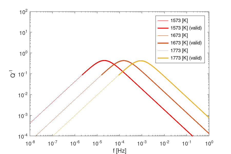
In addition to the usual outputs, the linear backstress model includes a calculation of the model’s characteristic angular frequency, omega_o, for each thermodynamic state. The corresponding output, valid_f, is a boolean matrix of the same shape as the frequency-dependent variables where the value is 1 if when the frequency is greater than omega_o / 10, indicating the regions where the linearized model is expected to be a good fit for the full backstress model (see Hein et al., 2025). This allows you to plot or highlight just the regions that are valid, e.g., see the cookbook example, CB_017_backstress_model.m:
Parameters
To view the full list of parameters,
VBR.in.anelastic.backstress_linear = Params_Anelastic('backstress_linear');
disp(VBR.in.anelastic.backstress_linear)
copying only relevant ones:
    func_name = Q_backstress_linear
    citations =
    {
      [1,1] = Hein et al., 2025, ESS Open Archive (Submitted to JGR Solid Earth ), https://doi.org/10.22541/essoar.174326672.28941810/v1
    }

    description = Linearized backstress model.
    sig_p_sig_dc_factor = 0.8000
    burgers_vector_nm = 0.5000
    Beta = 2
    Q_J_per_mol = 450000
    A = 8.7096e+06
    pierls_barrier_GPa = 3.1000
    G_UR = 65
    M_GPa = 135
    SV_required =
    {
      [1,1] = T_K
      [2,1] = sig_MPa
      [3,1] = dg_um
    }
Some notes on the above fields (see Hein et al, 2025 for more details):
sig_p_sig_dc_factor: the stress ratio of Taylor stress to bias stressM_GPa: the hardening modulusQ_J_per_mol: activation energy,dFused by Hein et al.Beta: geometric factorA: arrhensious pre-exponentional factor for low-temperature plasticityG_UR: is the fixed shear modulus, not actually used by the VBRc but included here for reference. The VBRc uses output from the anharmonic calculation.