eburgers_psp
Extended Burgers Model with Pseudo-Period Scaling, following Jackson and Faul (2010), Phys. Earth Planet. Inter., DOI. The default fitting parameters used are those of the multi-sample extended burgers fit (see below for other otpions).
Requires
The following state variable arrays are required:
VBR.in.SV.T_K % temperature [K]
VBR.in.SV.P_GPa % pressure [GPa]
VBR.in.SV.dg_um % grain size [um]
VBR.in.SV.sig_MPa % differential stress [MPa]
VBR.in.SV.phi % melt fraction / porosity
VBR.in.SV.rho % density in kg m<sup>-3</sup>
Additionally, eburgers_psp relies on output from the elastic methods so anharmonic MUST be in the VBR.in.elastic.methods_list. If anh_poro is in the methods list then eburgers_psp will use the unrelaxed moduli from anh_poro (which includes the P,T projection of anharmonic plus the poroelastic correction). See the section on elastic methods for more details.
Calling Procedure
% set required state variables
clear
VBR.in.SV.T_K=700:50:1200;
VBR.in.SV.T_K=VBR.in.SV.T_K+273;
sz=size(VBR.in.SV.T_K); % temperature [K]

% remaining state variables (ISV)
VBR.in.SV.dg_um=3.1*ones(sz);
VBR.in.SV.P_GPa = 0.2 * ones(sz); % pressure [GPa]
VBR.in.SV.rho = 3300 * ones(sz); % density [kg m^-3]
VBR.in.SV.sig_MPa = 10 * ones(sz); % differential stress [MPa]
VBR.in.SV.phi = 0.0 * ones(sz); % melt fraction

% set frequency range
VBR.in.SV.f = 1./logspace(-2,4,100);

% set elastic methods list (at least 'anharmonic' is required)
VBR.in.elastic.methods_list={'anharmonic';'anh_poro'};

% set anelastic methods list
VBR.in.anelastic.methods_list={'eburgers_psp'};

% call VBR_spine
[VBR] = VBR_spine(VBR) ;
Output
Output is stored in VBR.out.anelastic.eburgers_psp:
>> disp(fieldnames(VBR.out.anelastic.eburgers_psp))

{
  [1,1] = J1    % real part of dynamic compliance [1/Pa]
  [2,1] = J2    % complex part of dynamic compliance [1/Pa]
  [3,1] = Q     % quality factor
  [4,1] = Qinv  % attenuation
  [5,1] = M     % modulus [Pa]
  [6,1] = V     % shear wave velocity [m/s]
  [7,1] = tau_M % steady state maxwell time [s]
  [8,1] = Vave  % frequency-averaged shear wave velocity [m/s]
}
The following fields are frequency dependent: J1,J2,Q,Qinv,M and V.
Parameters
To view the full list of parameters,
VBR.in.anelastic.eburgers_psp = Params_Anelastic('eburgers_psp');
disp(VBR.in.anelastic.eburgers_psp)
Several import fields of VBR.in.anelastic.eburgers_psp include:
eBurgerFit: This field specifies which parameter fitting from Jackson and Faul (2010) to use. The possible values include:bg_only: (default) multi-sample fit for the high temperature background onlybg_peak: multi-sample fit for the high temperature background plus a dissipation peaks6585_bg_only: single sample fit for the high temperature background onlys6585_bg_peak: single sample fit for the high temperature background plus a dissipation peak
method: This field determines the method of calculating the integral within the relationship for real/complex dynamic compliances. The default valuePointWiseis a standard numerical integration. If set toFastBurger, the integral is computed using a look-up table approach. While theFastBurgeris significantly more efficient computationally, it only works when the dissipation peak is not included in the formulation.
To change the actual fitting parameters in VBR.in.anelastic.eburgers_psp.(fit), you should first load the parameter set and then modify values before calling the VBR Calculator. For example, to change the strength of the dissipation peak for the background and peak fit, bg_peak:
VBR.in.anelastic.eburgers_psp=Params_Anelastic('eburgers_psp');
VBR.in.anelastic.eburgers_psp.eBurgerFit='bg_peak'; % select the bg + peak
disp(VBR.in.anelastic.eburgers_psp.bg_peak.DeltaP) % print the default peak strength (0.057)
VBR.in.anelastic.eburgers_psp.bg_peak.DeltaP=.07; % increase peak strength
disp(VBR.in.anelastic.eburgers_psp.bg_peak.DeltaP)
on the reference modulus
The parameter fits include a value for the reference modulus, temperature and pressure. In the case of the bg_peak fit, these are:
G_UR =  66.500
TR =  1173
PR =  0.20000
which reflect the experimental conditions.
It is important to stress that these values are not used by the anharmonic calculation (as a result the reference modulus here is not used anywhere). The reference temperature and pressure are only used in calculating maxwell times when calculating the effective diffusion creep viscosity and do not match the reference values used by the anharmonic methods. In order to use the exact unrelaxed reference modulus of Jackson and Faul, 2010, you must either (1) overwrite VBR.in.elastic.anharmonic.Gu_0_ol using the JF10 value projected to the surface, as done in Projects/1_LabData/1_Attenuation/FitData_FJ10_eBurgers.m or (2) set VBR.in.elastic.anharmonic.Gu_0_ol to the exact JF10 value but then change VBR.in.elastic.anharmonic.T_K_ref and VBR.in.elastic.anharmonic.P_Pa_ref to match the the JF10 values.
Example at Laboratory Conditions
The script Projects/1_LabData/1_Attenuation/FitData_FJ10_eBurgers.m calculates the modulus, M, and attenuation, Q-1, for a temperature range of 700-1200oC in 50oC increments for periods in 10-2 to 104 s using the single sample fitting parameters for sample 6585 following Jackson and Faul (2010):
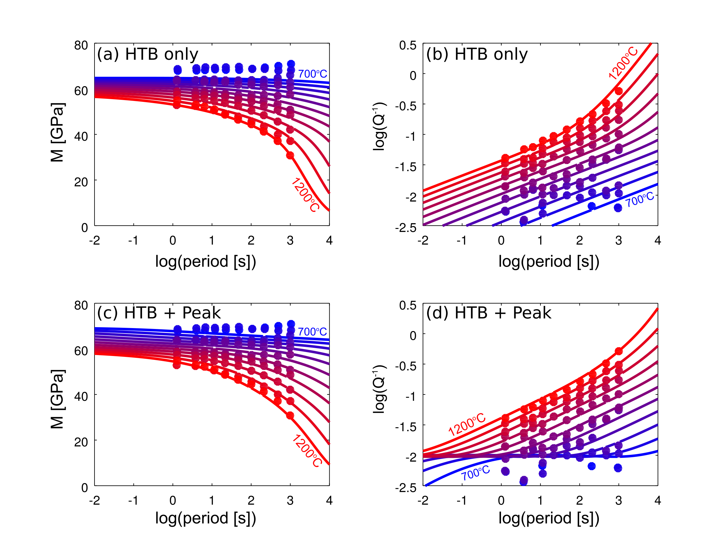
The top row (panels a and b) use the fitting parameters for the high temperature background only while the bottom row uses the fitting parameters when an additional dissipation peak is included. Data are from figure 1a-1d of Jackson and Faul 2010 and are not included in the present repository. The single sample fits are selected by setting the eBurgerFit parameter. For the background only,
VBR.in.anelastic.eburgers_psp.eBurgerFit='s6585_bg_only';
while for the background plus dissipation peak,
VBR.in.anelastic.eburgers_psp.eBurgerFit='s6585_bg_peak';