xfit_mxw

Master curve maxwell scaling falling McCarthy, Takei and Hiraga (2011) JGR, DOI.

Requires

The following state variable arrays are required:

VBR.in.SV.T_K % temperature [K]
VBR.in.SV.P_GPa % pressure [GPa]
VBR.in.SV.dg_um % grain size [um]
VBR.in.SV.sig_MPa % differential stress [MPa]
VBR.in.SV.phi % melt fraction / porosity
VBR.in.SV.rho % density in kg m<sup>-3</sup>

Additionally, xfit_mxw relies on output from the elastic methods and viscous methods.

Required Elastic Methods: anharmonic MUST be in the VBR.in.elastic.methods_list. If anh_poro is in the methods list then xfit_mxw will use the unrelaxed moduli from anh_poro (which includes the P,T projection of anharmonic plus the poroelastic correction). See the section on elastic methods for more details.

Required Viscous Methods: xfit_mxw relies on a viscosity relationship to calculate maxwell times. If none is set in VBR.in.viscous.methods_list then the VBR Calculator will use HZK2011. To use a different method, set VBR.in.viscous.methods_list={'HK2003'}. If multiple viscous methods are set, only the first will be used by xfit_mxw.

Calling Procedure

% set required state variables
clear
VBR.in.SV.T_K=700:50:1200;
VBR.in.SV.T_K=VBR.in.SV.T_K+273;
sz=size(VBR.in.SV.T_K); % temperature [K]

% remaining state variables (ISV)
VBR.in.SV.dg_um=3.1*ones(sz);
VBR.in.SV.P_GPa = 0.2 * ones(sz); % pressure [GPa]
VBR.in.SV.rho = 3300 * ones(sz); % density [kg m^-3]
VBR.in.SV.sig_MPa = 10 * ones(sz); % differential stress [MPa]
VBR.in.SV.phi = 0.0 * ones(sz); % melt fraction

% set frequency range
VBR.in.SV.f = 1./logspace(-2,4,100);

% set elastic methods list (at least 'anharmonic' is required)
VBR.in.elastic.methods_list={'anharmonic';'anh_poro'};
VBR.in.viscous.methods_list={'HZK2011'};

% set anelastic methods list
VBR.in.anelastic.methods_list={'xfit_mxw'};

% call VBR_spine
[VBR] = VBR_spine(VBR) ;

Output

Output is stored in VBR.out.anelastic.xfit_mxw:

>> fieldnames(VBR.out.anelastic.xfit_mxw)
ans =
{
  [1,1] = J1       % real part of dynamic compliance [1/Pa]
  [2,1] = J2       % complex part of dynamic compliance [1/Pa]
  [3,1] = Q        % quality factor
  [4,1] = Qinv     % attenuation
  [5,1] = M        % modulus [Pa]
  [6,1] = V        % shear wave velocity [m/s]
  [7,1] = f_norm   % normalized frequency
  [8,1] = tau_norm % normalized period
  [9,1] = tau_M    % maxwell time
  [10,1] = Vave    % frequency-averaged shear wave velocity [m/s]
}

The following fields are frequency dependent: J1,J2,Q,Qinv,M, V, f_norm, tau_norm.

Parameters

To view the full list of parameters,

VBR.in.anelastic.xfit_mxw = Params_Anelastic('xfit_mxw');
disp(VBR.in.anelastic.xfit_mxw)

Any of the parameters can be set before calling VBR_spine.

One parameter of particular note is VBR.in.anelastic.xfit_mxw.fit, which can be either fit1 (default) or fit2, which correspond to the two fits presented in McCarthy et al. 2011. fit1 is the fit that passes through the estimate of the relaxation spectrum from PREM at seismic frequencies while fit2 is a better fit to J1 and J2 of borneol at experimental conditions.

Example at Laboratory Conditions

The Project script, Projects/1_LabData/1_Attenuation/FitData_McCT11.m calculates J1 and J2 normalized by unrelaxed modulus vs. maxwell-normalized period for borneol following McCarthy et al. 2011:

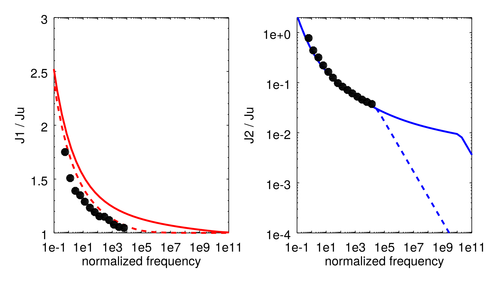
Data are from figure 15 of McCarthy et al. 2011 and are not included in the repository. The solid and dashed lines are fit 1 and fit 2, respectively.